插入的图片不能显示在正确位置

```tex \documentclass[12pt,a4]{article} %%%%%%%%%%%%%%%%%%%%%%%%%%%%%%%%%%%%%%%%%%%%%%%%%%%%%%%%%%%%%%%%%%%%%%%%%%%%%%%%%%%%%%%%%%%%%%%%%%%%%%%%%%%%%%%%%%%%%%%%%%%%%%%%%%%%%%%%%%%%%%%%%%%%%%%%%%%%%%%%%%%%%%%%%%%%%%%%%%%%%%%%%%%%%%%%%%%%%%%%%%%%%%%%%%%%%%%%%%%%%%%%%%%%%%%%%%%%%%%%%%%%%%%%%%%% \usepackage{amsfonts} \usepackage{amsthm} \usepackage{amsmath,mathrsfs} \usepackage{amssymb} \usepackage{graphicx} \usepackage{subfig} \usepackage{cite} \setcounter{MaxMatrixCols}{10} %TCIDATA{OutputFilter=LATEX.DLL} %TCIDATA{Version=5.00.0.2606} %TCIDATA{} %TCIDATA{BibliographyScheme=Manual} %TCIDATA{LastRevised=Monday, April 29, 2013 16:28:32} %TCIDATA{} %TCIDATA{Language=American English} \topmargin -0.5cm \oddsidemargin -0.5cm \evensidemargin -0.5cm \textwidth=17 true cm \textheight=23.2 true cm %\input{tcilatex} \begin{document} \title{ Parallel *** in Hilbert space } \author{*** $^{1,}$\thanks{Corresponding author.}, ??? $^2$ \\ \\ \footnotesize{$^1$ Department of Mathematics, *** University}\\ \footnotesize{ ***, China}\\ \footnotesize{ $^2$ Department of Engineering, *** University}\\ \footnotesize{ ***, China}\\ \\ \\ \\ \footnotesize{ E-mails: ???@163l.com} } \date{} \maketitle {\footnotesize \noindent \textbf{Abstract.} \vskip 0.2cm } {\footnotesize \noindent \textbf{Keywords}: .\vskip 1mm } {\footnotesize \noindent \textbf{2010 AMS Subject Classification}: } \vskip 4mm \section*{1. Introduction} \vskip 0.5cm \section*{2. Preliminaries}\vskip 2mm \section*{3. Main results} \vskip0.3cm \newpage where $\{\alpha_n\}\subset(0,1)$, $\rho\in(0,\min\{\frac{1}{2c_1},\frac{1}{2c_2}\}$. If $\lim_{n\to\infty}\alpha_n=0$, then $\{x_n\}$ generated by $(3.20)$ converges strongly to element $\hat{x}=P_\Omega x_1.$ \vskip0.2cm \noindent {\bf Remark 3.2} If $U_i\equiv U$ for each $i=1,\ldots, N$ and $V_j\equiv V$ for each $j=1,\ldots, M$ in Theorems 3.1 and 3.2, we obtain the corresponding results announced in \cite[Theorem 1,Theorem 2]{HieuMuuAnh2016}. \vskip0.2cm \section*{4. Numerical experiment} \vskip0.2cm In this section, we give an example to illustrate the algorithms in this paper. We perform the algorithms by Matlab R2008a running on a PC Desktop with Core(TM) i3CPU M550 3.20GHz with 4GB Ram. \vskip0.2cm \noindent {\bf Example 4.1} Let $H=\mathbb{R}^3$ and $U_1=\{(x_1,x_2,x_3): x_1\in[0,1], x_2\geq 0,x_3\geq 0\}$, $U_2=\{(x_1,x_2,x_3): x_1\geq 0,x_2\in[0,2], x_3\geq 0\}$ and $U_3=\{(x_1,x_2,x_3): x_1\geq 0,x_2\geq 0, x_3\in[0,3]\}$. For each $i=1,2,3$, let $f_i(x,y)=(y_i-x_i)\|x\|$ for all $x=(x_1,x_2,x_3), y=(y_1,y_2,y_3)\in U_i$. From \cite{Wang2018} it follows that each $f_i$ satisfies the conditions (i)-(iv) with the Lipschitz constants $c_1=c_2=1$. Let $V_j=\{(x_1,x_2,x_3): x_1\in\mathbb{R}, 0\leq x_2\leq j,x_3\geq 0\}$ for each $j=1,\ldots,M$. Define the nonexpansive mapping $S_j$ on $V_j$ by $S_jx=(-\frac{x_1}{2}, \frac{x_2^2}{6j},\frac{x_3}{2})$ for $j=1,\ldots,M$. Obviously, $\mathcal{F}=\cap_{i=1}^3 EP(f_i)\cap(\cap_{j=1}^M)Fix(S_j)=\{(0,0,0)\}$. 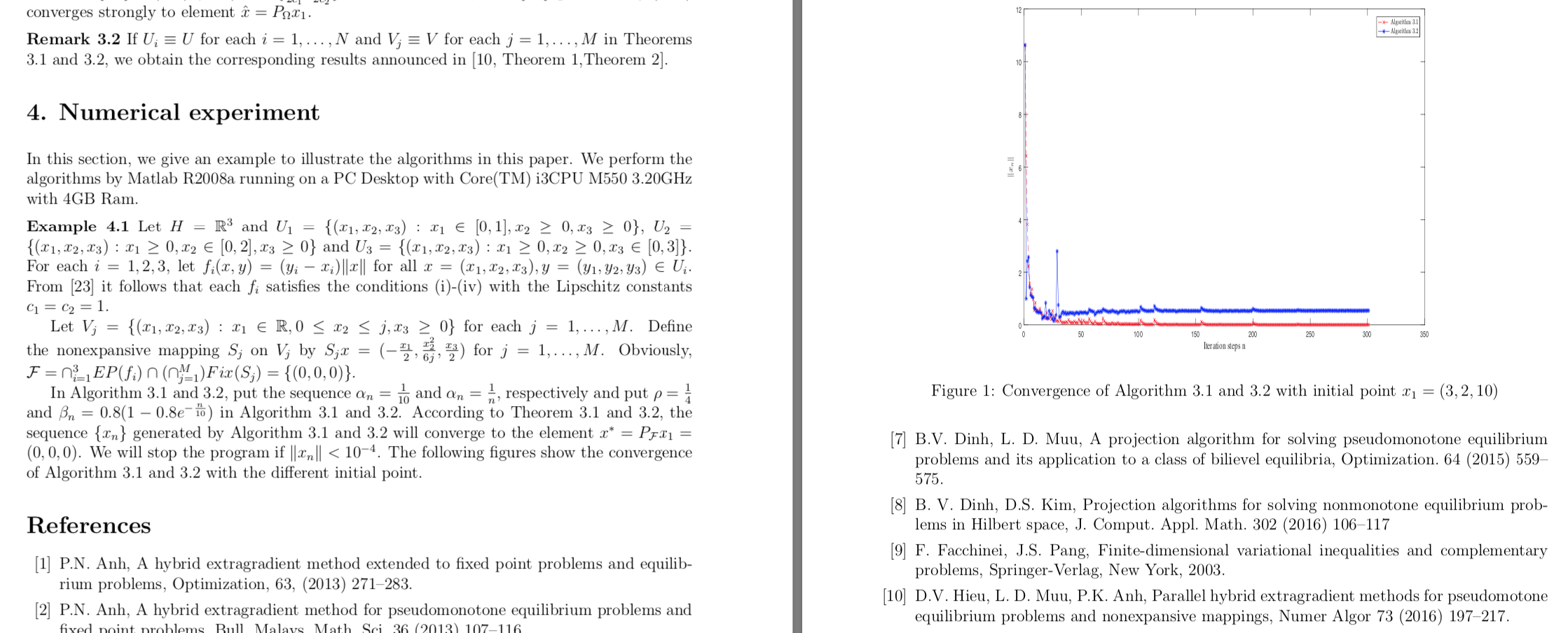In Algorithm 3.1 and 3.2, put the sequence $\alpha_n=\frac{1}{10}$ and $\alpha_n=\frac{1}{n}$, respectively and put $\rho=\frac{1}{4}$ and $\beta_n= 0.8(1-0.8 e^{-\frac{n}{10}})$ in Algorithm 3.1 and 3.2. According to Theorem 3.1 and 3.2, the sequence $\{x_n\}$ generated by Algorithm 3.1 and 3.2 will converge to the element $x^*=P_{\mathcal{F}}x_1=(0,0,0)$. We will stop the program if $\|x_n\|<10^{-4}$. The following figures show the convergence of Algorithm 3.1 and 3.2 with the different initial point. \begin{figure}[h] \centering \subfloat {% \includegraphics[width=5.2in,totalheight=3.9in]{a1.eps}}\ \caption{ Convergence of Algorithm 3.1 and 3.2 with initial point $x_1=(3,2,10)$} \end{figure} \iffalse \section*{Acknowledgments} \vskip0.2cm This work is supported by Natural Science Foundation of Hebei Province (N0. A2015502021) and the Fundamental Research Funds for the Central Universities (No. 2015MS78). \fi \begin{thebibliography}{99} \setlength{\itemsep}{-0.02cm} \bibitem{Anh2013}P.N. Anh, A hybrid extragradient method extended to fixed point problems and equilibrium problems, Optimization, 63, (2013) 271--283. \bibitem{Anh2013-2}P.N. Anh, A hybrid extragradient method for pseudomonotone equilibrium problems and fixed point problems, Bull. Malays. Math. Sci. 36 (2013) 107--116. \bibitem{AhnThi2013}P.N. Anh, H.A. Le Thi, An Armijo-type method for pseudomonotone equilibrium problems and its applications, J. Glob. Optim. 57 (2013) 803--820. %\bibitem{Bnouhachem2014}A. Bnouhachem, Strong convergence algorithm for split equilibrium problems and hierarchical fixed point problems, The Scientific World Journal, 2014, Article ID 390956, 12 pages. %\bibitem{Ceng2008}L.C. Ceng, P. Cubiotti, J.C. Yao, {\it An implicit iterative scheme for monotone variational inequalities and fixed point problems}, % Nonlinear Anal., {\bf69}, (2008), 2445--2457. % \bibitem{CensorBibaliReich2012}Y. Censor, A. Gibali, S. Reich, Algorithms for the split variational inequality problem, Number Algor. 59 (2012) 301--323 \bibitem{ChangLeeChan2009}S.-S. Chang, H. W. J. Lee, and C. K. Chan, A new method for solving equilibrium problem fixed point problem and variational inequality problem with application to optimization, Nonlinear Analysis, Theory, Methods and Applications, 70 (2009) 3307--3319. %\bibitem{ChoZhou2004}Y. J. Cho, H.Y. Zhou and G.T. Guo, Weak and strong convergence theorems for three-step iterations with errors for asymptotically nonexpansive mappings, Comput. Math. Appl. 47 (2004) 707--717. \bibitem{CombettesHirstoaga1997}P. L. Combettes, S. A. Hirstoaga, Equilibrium programming using proximal like algorithms, Mathematical Prog. 78 (1997) 29--41. \bibitem{CombettesHirstoaga2005}P.L. Combettes, S.A. Hirstoaga, Equilibrium programming in Hiblert spaces, J. Nonlinear Convex Anal. 6 (2005) 117--136. \bibitem{DinhMuu2015}B.V. Dinh, L. D. Muu, A projection algorithm for solving pseudomonotone equilibrium problems and its application to a class of bilievel equilibria, Optimization. 64 (2015) 559--575. \bibitem{DinhKim2016}B. V. Dinh, D.S. Kim, Projection algorithms for solving nonmonotone equilibrium problems in Hilbert space, J. Comput. Appl. Math. 302 (2016) 106--117 \bibitem{FacchineiPang2003}F. Facchinei, J.S. Pang, Finite-dimensional variational inequalities and complementary problems, Springer-Verlag, New York, 2003. % \bibitem{FangHuang2003}Y.P. Fang, N.J. Huang, Variational-like inequilities with generalized %monotone mappings in Banach spaces, J. Optim. Theory Appl. 118 (2003) 327--338. \bibitem{HieuMuuAnh2016}D.V. Hieu, L. D. Muu, P.K. Anh, Parallel hybrid extragradient methods for pseudomotone equilibrium problems and nonexpansive mappings, Numer Algor 73 (2016) 197--217. %\bibitem{IidukaTakahashi2005} H. Iiduka, W. Takahashi, Strong convergence theorems for nonexpansive mappings and inverse-strongly monotone mappings, Nonlinear Anal. (61) (2005) 341--350. \bibitem{KangChoLiu2010}S.M. Kang, S.Y. Cho, Z. Liu, Convergence of iterative sequences for generalized equilibrium problems involving inverse-strongly monotone mappings. J. Inequal. Appl. 2010, 827082 (2010) \bibitem{KatchangKumam2010} P. Katchang and P. Kumam, A new iterative algorithm of solution for equilibriumproblems, variational inequalities and fixed point problems in a Hilbert space, Journal of Applied Mathematics and Computing, 32 (2010) 19--38. %\bibitem{KazmiRizvi2013}K. R. Kazmi and S. H. Rizvi, Iterative approximation of a %common solution of a split equilibrium problem, a variational %inequality problem and a fixed point problem, Journal of the %Egyptian Math. Society 21 (2013) 44--51. %\bibitem{Liu1995} L.S. Liu, Iterative processes with errors for nonlinear strongly accretive mappings in Banach spaces, J. Math. Anal.% %Appl. 194 (1995) 114--125. %\bibitem{Mainge2007} P.E. Maing\'{e}, Approximation methods for common fixed points of nonexpansive mappings in Hilbert spaces, J. Math. Anal. Appl. vol. 325 (2007), 469--479. \bibitem{Mainge2008} P.E. Maing\'{e}, Strong convergence of projected subgradient methods for nonsmooth and nonstrictly convex minimization, Set-Valued Anal. 16 (2008) 899--912. %\bibitem{Moudafi2011} A. Moudafi, Split Monotone Variational Inclusions, J. Optim Theory %Appl. 150 (2011) 275--283. \bibitem{PlubtiengPunpaeng2007} S. Plubtieng and R. Punpaeng, A general iterative method for equilibrium problems and fixed point problems in Hilbert spaces, J. Math. Anal. Appl. 336 (2007) 455--469. \bibitem{QinChoKang2010}X. Qin, Y.J. Cho, S.M. Kang, Viscosity approximation methods for generalized equilibrium problems and fixed point problems with applications. Nonlinear Anal. 72, 99--112 (2010) \bibitem{QinShangSu2008} X. Qin, M. Shang, and Y. Su, A general iterative method for equilibrium problems and fixed point problems in Hilbert spaces, Nonlinear Anal. 69 (2008) 3897--3909. % \bibitem{Suzuki2005}T. Suzuki, Strong convergence of Krasnoselskii and Mann's type sequences for one-parameter nonexpansive semigroups without Bochner integrals, J. Math. Anal. Appl. 305 (2005) 227--239. % \bibitem{Takahashi2000}W. Takahashi, Nonlinear Functional Analysis, Yokohama Publishers, Yokohama, 2000. \end{thebibliography} \end{document} ``` 希望插入的图片在参考文献和The following figures show the 。。之间，也就是图片1中黑色箭头位置，但编译完后却出现在图2位置， 代码处已经添加了参数h了。图a1.esp 不知道怎么上传。只上传了图1和2